Validation of SVI results

This is a quick reference and validation of our functions to calculate SVI from Census data, where we’ll include the tables for retrieving census variables and normalizing data, as well as a comparison between findSVI calculations and CDC/ATSDR SVI data.

library(findSVI)
library(dplyr)
library(tidyr)
library(reactable)
library(stringr)
library(purrr)
library(ggplot2)

SVI variables and Census variables

For each year between 2012-2021, we include a dataset in the package containing the SVI variable names, their theme group and corresponding Census variable(s) and calculation formula. The information is extracted from CDC/ATSDR SVI documentation for the years available, and modified for the years that the CDC/ATSDR SVI database does not cover (if Census variable names are different, otherwise information of the adjacent year is used). These datasets are documented in ?variable_calculation.

datasets <- list( 
  variable_e_ep_calculation_2012,
  variable_e_ep_calculation_2013,
  variable_e_ep_calculation_2014,
  variable_e_ep_calculation_2015,
  variable_e_ep_calculation_2016,
  variable_e_ep_calculation_2017,
  variable_e_ep_calculation_2018, 
  variable_e_ep_calculation_2019,
  variable_e_ep_calculation_2020,
  variable_e_ep_calculation_2021
)

process_file <- function(file) {
  data_tmp <- file
  year_info <- colnames(file)
  
  data_tmp %>% 
    mutate(year = str_sub(year_info[1], 2, 5), .before = 1) %>% 
    rename(SVI_var = 2,
    Theme = 3,
    Census_var = 4) 
}
  
all_datasets <- datasets %>% 
  map(process_file) %>% 
  list_rbind()

Here we show all the datasets as one table for easier search and reference, with the columns represent:

year: The year that the other columns of data correspond to.
SVI_var: SVI variable names (“E_xx” for counts, “EP_xx” for normalized values).
Theme: SVI variables are categorized into four themes/domains: 1) Socioeconomic Status, 2) Household Characteristics, 3) Racial & Ethnic Minority Status and 4) Housing Type/Transportation. Theme 0 is used for 3 variables representing total counts, while theme 5 is used for adjunct variables (not included in calculation).
Census_var: Census variable name(s) corresponding to the SVI variable, and/or the calculation using SVI/census variables.

reactable(
  all_datasets,
  filterable = TRUE,
  searchable = TRUE,
  resizable = TRUE,
  bordered = TRUE,
  minRows = 10,
  highlight = TRUE,
  showPageSizeOptions = TRUE,
  pageSizeOptions = c(10,20,30),
  defaultPageSize = 10
)

Correlation between CDC/ATSDR and findSVI results

As part of the automatic unit testing in the package, county-level SVI calculations for Pennsylvania for 2014, 2016, 2018 and 2020 are compared with the SVI results downloaded from CDC/ATSDR SVI database and the tests are considered passed when correlation coefficient is higher than 0.9995.

For example, comparing two versions of SVIs for 2020:

#source:https://www.atsdr.cdc.gov/placeandhealth/svi/data_documentation_download.html
#rename FIPS to GEOID
load(system.file("testdata","cdc_pa_cty_svi2020.rda",package = "findSVI"))

#Census API key required for raw data retrieval
pa_cty_raw <- load(system.file("testdata","pa_cty_raw2020.rda",package = "findSVI")) %>%
    get()

output <- get_svi(2020, pa_cty_raw)

join_RPL <- cdc_pa_cty_svi2020 %>%
    select(GEOID,
      cdc_RPL_themes = RPL_THEMES,
      cdc_RPL_theme1 = RPL_THEME1,
      cdc_RPL_theme2 = RPL_THEME2,
      cdc_RPL_theme3 = RPL_THEME3,
      cdc_RPL_theme4 = RPL_THEME4) %>%
    mutate(GEOID = paste(GEOID)) %>%
    left_join(output %>%
        select(GEOID,
          RPL_themes,
          RPL_theme1,
          RPL_theme2,
          RPL_theme3,
          RPL_theme4)) %>%
    drop_na() %>%   ## remove NA rows
    filter_all(all_vars(. >= 0)) #-999 in cdc data
#> Joining with `by = join_by(GEOID)`

coeff1 <- cor(join_RPL$cdc_RPL_themes, join_RPL$RPL_themes)

join_RPL %>% 
  ggplot(aes(x = cdc_RPL_themes, y = RPL_themes)) +
  geom_point(color = "#004C54")+
  geom_abline(slope = 1, intercept = 0)+
  labs(title = "CDC vs. findSVI CTY-level SVI for Pennsylvania in 2020",
    subtitle = paste0("Comparison of overall percentile ranking (RPLs), correlation coefficient = ", coeff1),
    y = "findSVI",
    x = "CDC")+
  theme(plot.title = element_text(size= 15))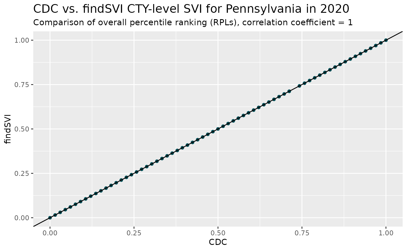

Similarly, we could visualize the two versions of census tract-level SVIs for Delaware for 2020. (For considerations of datasets size in the package, census tract-level SVI comparisons are not included in the automated testing.)

load(system.file("extdata","cdc_de_ct_svi2020.rda",package = "findSVI"))

de_ct_raw <- load(system.file("extdata","de_ct_raw2020.rda",package = "findSVI")) %>%
    get()

output2 <- get_svi(2020, de_ct_raw)

join_RPL2 <- cdc_de_ct_svi2020 %>%
    select(GEOID,
      cdc_RPL_themes = RPL_THEMES,
      cdc_RPL_theme1 = RPL_THEME1,
      cdc_RPL_theme2 = RPL_THEME2,
      cdc_RPL_theme3 = RPL_THEME3,
      cdc_RPL_theme4 = RPL_THEME4) %>%
    mutate(GEOID = paste(GEOID)) %>%
    left_join(output2 %>%
        select(GEOID,
          RPL_themes,
          RPL_theme1,
          RPL_theme2,
          RPL_theme3,
          RPL_theme4)) %>%
    drop_na() %>%   ## remove NA rows
    filter_all(all_vars(. >= 0)) #-999 in cdc data
#> Joining with `by = join_by(GEOID)`

coeff2 <- round(cor(join_RPL2$cdc_RPL_themes, join_RPL2$RPL_themes),6)

join_RPL2 %>% 
  ggplot(aes(x = cdc_RPL_themes, y = RPL_themes)) +
  geom_point(color = "#004C54")+
  geom_abline(slope = 1, intercept = 0)+
  labs(title = "CDC vs. findSVI CT-level SVI for Delaware in 2020",
    subtitle = paste0("Comparison of overall percentile ranking (RPLs), correlation coefficient = ", coeff2),
    y = "findSVI",
    x = "CDC")+
  theme(plot.title = element_text(size= 15))

SVI variables and Reproducing CDC/ATSDR SVI

SVI variables and Census variables

Correlation between CDC/ATSDR and findSVI results